Prévisions étranges avec ARMA

Le problème exposé dans ce sujet a été résolu.

Bonjour,

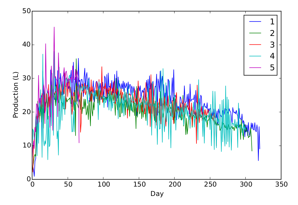
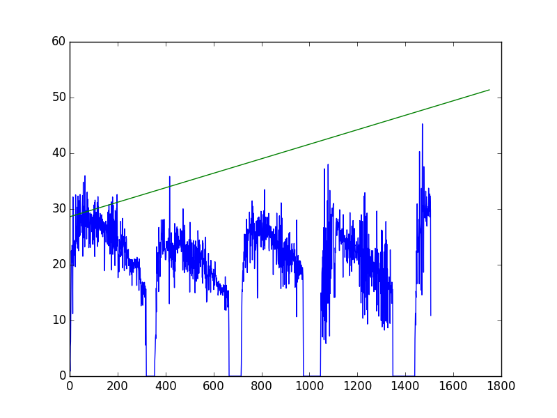
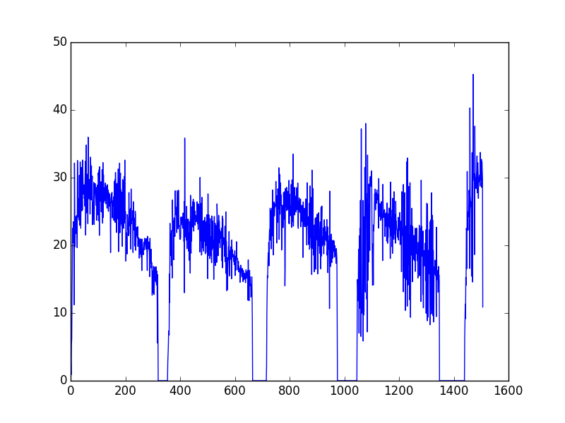
Je travaille sur la série temporelle suivante :

1
3.89, 2.81, 0.88, 5.36, 6.18, 12.05, 16.16, 22.52, 20.4, 21.87, 23.48, 23.01, 19.4, 11.21, 32.16, 26.33, 19.8, 23.09, 21.73, 24.25, 23.18, 22.03, 24.42, 23.11, 19.65, 32.53, 28.42, 24.18, 26.41, 26.9, 23.85, 23.73, 30.35, 22.98, 24.2, 32.32, 27.96, 22.51, 26.69, 31.51, 28.69, 25.09, 28.5, 25.24, 32.61, 30.26, 27.78, 27.56, 28.5, 28.96, 26.92, 27.75, 25.8, 30.38, 32.43, 21.51, 28.34, 34.82, 24.79, 28.19, 30.36, 25.02, 30.54, 23.21, 35.98, 29.04, 29.48, 26.87, 29.68, 29.74, 28.66, 24.62, 30.26, 33.03, 26.76, 30.7, 31.75, 26.69, 29.41, 30.24, 23.05, 26.26, 23.82, 26.43, 26.58, 29.29, 23.09, 26.85, 27.73, 29.02, 29.12, 28.39, 26.98, 25.9, 27.13, 28.56, 23.69, 27.72, 28.91, 26.36, 24.5, 30.71, 30.04, 23.62, 31.15, 21.46, 31.61, 27.43, 27.68, 26.51, 27.07, 29.4, 24.95, 28.81, 25.43, 31.19, 25.28, 23.27, 32.23, 24.1, 30.44, 26.32, 28.49, 27.56, 26.62, 28.45, 26.91, 29.21, 26.14, 28.77, 27.2, 27.7, 28.63, 25.5, 28.97, 26.9, 28.14, 28.19, 25.02, 27.78, 27.01, 25.81, 27.58, 26.08, 26.4, 24.32, 18.93, 26.96, 27.18, 27.6, 26.27, 27.83, 24.05, 25.7, 26.53, 25.83, 26.65, 27.18, 23.69, 25.74, 29.46, 25.95, 29.75, 23.39, 30.77, 26.79, 28.94, 28.3, 21.9, 29.14, 23.89, 26.41, 27.76, 27.4, 31.28, 19.06, 29.87, 28.61, 26.09, 32.15, 21.86, 29.09, 30.67, 25.15, 28.19, 23.17, 25.69, 22.86, 27.85, 19.84, 29.73, 29.48, 24.2, 24.93, 22.51, 26.08, 30.18, 23.3, 32.6, 23.99, 25.04, 24.52, 17.67, 21.86, 21.11, 21.72, 18.73, 24.54, 24.22, 22.98, 22.4, 22.18, 21.42, 27.8, 22.94, 22.86, 23.25, 25.28, 21.67, 25.46, 19.43, 28.33, 23.16, 23.67, 23.84, 23.87, 23.75, 25.13, 18.94, 26.45, 22.95, 22.98, 22.25, 23.43, 24.01, 19.88, 25.03, 24.55, 19.26, 21.74, 21.62, 22.64, 21.5, 21.61, 21.12, 22.76, 19.83, 20.99, 20.27, 21.12, 20.74, 18.11, 20.12, 18.95, 20.92, 18.69, 20.94, 19.9, 18.26, 20.39, 16.27, 20.92, 19.82, 19.33, 19.08, 18.61, 18.64, 20.41, 20.47, 19.33, 21.04, 20.77, 20.74, 20.31, 19.89, 19.42, 21, 20.33, 20.05, 18.67, 16.28, 21.34, 20.13, 19.77, 20.05, 19.48, 20.5, 19.36, 18.91, 15.38, 21.05, 18.13, 18.13, 17.38, 19.42, 16.65, 17.48, 16.85, 12.63, 16.23, 14.08, 16.15, 12.99, 16.9, 13.95, 12.73, 14.52, 16.78, 14.97, 16.66, 14.81, 14.65, 16.84, 14.49, 14.14, 16.2, 14.44, 5.56, 15.66, 9.08, 0, 0, 0, 0, 0, 0, 0, 0, 0, 0, 0, 0, 0, 0, 0, 0, 0, 0, 0, 0, 0, 0, 0, 0, 0, 0, 0, 0, 0, 0, 0, 0, 0, 0, 0, 2.68, 3.75, 4.96, 6.92, 7.39, 6.74, 15.8, 11.52, 23.25, 18.49, 20.29, 18.84, 21.75, 17.02, 22.19, 20.56, 15.18, 26.7, 23.74, 22.15, 23.62, 22.26, 17.87, 24.05, 23.76, 22.22, 21.32, 28.06, 25.93, 24.82, 24.51, 25.62, 24.92, 21.88, 28.05, 23.77, 24.72, 22.87, 22.44, 28.15, 24.03, 22.78, 22.94, 22.65, 20.93, 20.98, 20.88, 21.23, 24.19, 23.01, 23.61, 23.69, 23.9, 24.2, 22.61, 22.53, 24.78, 23.86, 23.52, 20.54, 26.5, 13, 35.85, 22.43, 22.1, 21.24, 23.76, 23, 20.75, 25.76, 19.5, 21.47, 21.01, 23.88, 21.05, 23.82, 19.14, 19.87, 21.92, 17.77, 23.49, 20.75, 15.89, 27.4, 20.56, 18.85, 22.89, 20.63, 24.03, 25.72, 24.61, 26.45, 22.72, 26.81, 25.26, 22.1, 26.39, 25.19, 23.89, 25.07, 22.98, 23.94, 24.32, 24.42, 23.48, 24.41, 24.12, 26.43, 25.22, 23.16, 25.56, 22.33, 26.11, 24.71, 23.35, 25.76, 22.3, 19.03, 30.03, 22.56, 20.67, 26.2, 22.82, 18.56, 18.64, 27.1, 19.62, 22.48, 22.28, 20.9, 23.59, 19.14, 23.67, 21.42, 23.09, 20.59, 24.15, 18.75, 23.47, 20.53, 22.87, 20.54, 19.94, 24.52, 18.95, 22.66, 15.08, 27.61, 18.48, 20.79, 24.5, 19.44, 20.06, 23.02, 18.02, 23.95, 18.46, 21.28, 21.12, 20.06, 17.43, 24.34, 19.32, 21.53, 23.61, 19.6, 20.13, 20.76, 14.95, 21.49, 24.27, 19.21, 17.47, 23.26, 17.02, 20.08, 22.91, 21.46, 21.6, 17.48, 26.13, 23.97, 23.15, 21.21, 18.46, 20.43, 24.44, 20.36, 23.6, 22.02, 22.32, 19.65, 21.98, 22.05, 21.62, 21.02, 21.68, 22.55, 17.69, 24.33, 16.67, 23.93, 20.28, 20.12, 21.15, 20.88, 20.58, 18.78, 18.35, 22.82, 17.58, 18.02, 24.96, 15.84, 20.59, 18.16, 13.29, 18.18, 13.46, 15.67, 17.69, 17.98, 19.8, 17.96, 22.05, 15.48, 18.68, 19.17, 18.42, 18.77, 19.78, 17.92, 19.02, 15.05, 20.8, 18.34, 19.37, 18.32, 18.72, 18.36, 18.07, 17.61, 18.42, 17.15, 17.97, 19.2, 15.54, 17.62, 17.54, 18.44, 16.35, 20.54, 18.1, 18.07, 17.94, 18.08, 17.13, 16.36, 17.64, 16.11, 16.91, 16.07, 16.33, 16.57, 14.53, 15.02, 15.28, 17.07, 16.13, 16.61, 16.28, 15.41, 15.37, 16.57, 14.96, 14.63, 16.29, 15.31, 14.92, 15.38, 15.5, 15.9, 15.04, 15.47, 14.48, 15.53, 16.4, 15.12, 16.09, 16.09, 15.94, 15.58, 16.27, 11.89, 17.86, 13.93, 15.06, 11.82, 15.67, 16.32, 14.06, 15.34, 14.36, 14.18, 12.38, 12.74, 12.79, 15.35, 12.92, 8.44, 0, 0, 0, 0, 0, 0, 0, 0, 0, 0, 0, 0, 0, 0, 0, 0, 0, 0, 0, 0, 0, 0, 0, 0, 0, 0, 0, 0, 0, 0, 0, 0, 0, 0, 0, 0, 0, 0, 0, 0, 0, 0, 0, 0, 0, 0, 0, 0, 0, 0, 0, 2.2, 9.68, 12.48, 15.5, 15.2, 17.48, 18.88, 16.99, 20.43, 17, 21.2, 22.35, 20.74, 25.49, 21.52, 25.15, 23.37, 19.47, 20.82, 25.48, 23.11, 21.4, 28.18, 21.7, 24.6, 18.58, 24.77, 26.39, 24.34, 24.44, 25.7, 25.62, 26.1, 25.82, 29.45, 26.18, 26.91, 20.34, 27.3, 26.08, 23.38, 28.34, 27.04, 26.51, 25.4, 31.47, 20.88, 26.93, 30.49, 24.61, 28.54, 29.24, 25.94, 27.45, 25.27, 19.31, 21.28, 25.54, 25.93, 23.79, 22.62, 23.37, 27.8, 25.89, 23.87, 24.89, 27.94, 14.01, 16.97, 28.41, 27.9, 25.87, 25.65, 28.58, 25.13, 26.01, 28.01, 27.79, 27.14, 25.29, 27.41, 23.27, 29.6, 23.17, 27.56, 26.02, 25.59, 24.38, 25.1, 25.84, 29, 25.3, 22.66, 29.68, 23.5, 25.83, 24.1, 33.48, 22.84, 27.22, 27.57, 26.87, 28.56, 24.49, 27.09, 26.5, 25.49, 27.28, 24.91, 28.53, 25.25, 25.27, 27.14, 25.71, 29.22, 23.06, 22.5, 26.52, 25.01, 27, 26.08, 25.84, 24.83, 25.47, 26.83, 22.75, 25.94, 24.97, 23.52, 25.71, 24.19, 25.91, 25.27, 18.21, 26.42, 25.07, 25.42, 25.12, 23.43, 22.76, 25.47, 22.77, 23.77, 26.86, 22.89, 24.05, 23.75, 20.05, 29.26, 24.4, 23, 24.25, 23.63, 20.8, 20.12, 21.8, 26.24, 19.42, 19.78, 28.78, 21.18, 22.23, 23.68, 19.64, 27.1, 15.7, 31.12, 19.55, 19.59, 28.39, 23.87, 18.57, 19.45, 21.24, 16.09, 23.01, 19.96, 19.89, 23.99, 20, 16.47, 24.14, 20.82, 22.48, 22.13, 24.6, 19.59, 15.79, 20.97, 21.57, 24.82, 21.7, 19.98, 20.01, 18.82, 22.49, 23.47, 20, 16.52, 25.64, 18.4, 23.75, 25.81, 19.9, 21.24, 20.86, 20.15, 20.83, 22.61, 18.74, 21.41, 23.78, 20.01, 21.99, 22.74, 21.34, 20.86, 21.96, 21.33, 20.61, 23.82, 18.55, 19.11, 22.72, 15.95, 21.46, 19.43, 19.42, 20.64, 19.55, 10.66, 28.02, 21.03, 20.08, 16.87, 20.8, 20.07, 21.66, 17.44, 20.04, 18.64, 20.67, 18.11, 20.75, 19.1, 19.46, 20.66, 20.31, 18.27, 18.9, 19.95, 19.25, 18.98, 18.07, 17.33, 19.51, 18.68, 18, 10.02, 0, 0, 0, 0, 0, 0, 0, 0, 0, 0, 0, 0, 0, 0, 0, 0, 0, 0, 0, 0, 0, 0, 0, 0, 0, 0, 0, 0, 0, 0, 0, 0, 0, 0, 0, 0, 0, 0, 0, 0, 0, 0, 0, 0, 0, 0, 0, 0, 0, 0, 0, 0, 0, 0, 0, 0, 0, 0, 0, 0, 0, 0, 0, 0, 0, 0, 0, 0, 0, 0, 0, 0, 8.85, 14.95, 14.27, 11.8, 13.2, 18.53, 19.44, 7.03, 21.42, 10.71, 22.54, 19.66, 26.65, 19.55, 6.54, 37.22, 11.25, 9.95, 11.46, 10.43, 13.84, 26.63, 5.85, 18.81, 9.71, 10.22, 24.23, 15.91, 31.52, 25.16, 13.09, 38.02, 26.73, 27.69, 26.47, 12.04, 14.33, 7.21, 33.34, 14.82, 18.77, 25.99, 17.54, 29.07, 20.91, 24.77, 19.25, 29.67, 30.18, 28.7, 29.73, 28.83, 30.71, 31.01, 23.44, 18.97, 14.11, 14.27, 20.22, 14.15, 23.03, 22.12, 24.05, 25.68, 27.57, 26.49, 28.32, 25.23, 27.03, 27.74, 26.55, 26.23, 28.19, 26.75, 27.42, 27.53, 27.53, 25.06, 22.55, 29.88, 25.77, 24.26, 25.38, 26.16, 25.56, 25.47, 23.7, 26.17, 24.39, 26.47, 23.97, 24.23, 24.59, 17.74, 29.01, 25.59, 24.47, 24.21, 24.12, 24.2, 25.28, 21.32, 24.69, 22.75, 23.26, 23.94, 23.68, 24.84, 20.62, 26.27, 26.2, 20.3, 24.67, 21.17, 23.09, 22.83, 23.08, 25.52, 25.23, 22.55, 22.87, 18.05, 29.36, 21.4, 22.84, 22.72, 24.12, 19.8, 25.23, 18.81, 26.95, 22.92, 25.87, 22.51, 20.91, 27.93, 21.7, 23.65, 24.57, 21.73, 20.31, 26.52, 23.38, 23.56, 22.52, 22.36, 22.13, 21.19, 22.24, 22.11, 24.15, 20.78, 22.53, 22.24, 22.72, 23.28, 24.85, 20.11, 23.59, 22.54, 22.25, 23.28, 16.1, 27.93, 23.19, 21.5, 22.52, 22.38, 13.13, 28.99, 21.83, 21.82, 22.55, 15.19, 27.78, 20.58, 10.38, 22.24, 22.84, 14.92, 15.09, 32.32, 21.18, 11.02, 32.92, 17.06, 14.14, 18.27, 28.71, 17.15, 21.57, 20.9, 11.94, 29.27, 20.25, 9.36, 22.96, 18.54, 18.62, 20.39, 25.48, 21.72, 14.63, 22.8, 20.66, 19.15, 17.95, 21.46, 21.42, 17.74, 21.43, 19.3, 22.52, 16.14, 20.26, 21.93, 19.33, 22.54, 18.74, 20.49, 17.73, 19.12, 15.18, 19.05, 20.39, 18.64, 20.71, 22.96, 15.51, 18.95, 18.14, 20.18, 22.56, 11.7, 29.63, 18.4, 22.79, 18.46, 18.99, 19.29, 12.74, 22.11, 10.76, 19.27, 18.44, 16.94, 18.91, 19.06, 18.37, 20.34, 14.81, 22.29, 9.97, 17.93, 26.23, 18.03, 8.85, 26.12, 18.08, 9.4, 19.26, 17.14, 17.96, 15.82, 22.31, 16.08, 8.26, 23.51, 11.16, 23.77, 13.97, 9.88, 27.77, 10.47, 24.46, 11.21, 23.71, 9.61, 19.24, 15.56, 8.67, 16.79, 16.5, 16.6, 15.76, 17.82, 15.53, 15.83, 17.13, 9.47, 22.68, 15.89, 14.93, 16.28, 15.51, 15.35, 13.07, 16.88, 14.84, 15.63, 14.79, 0, 0, 0, 0, 0, 0, 0, 0, 0, 0, 0, 0, 0, 0, 0, 0, 0, 0, 0, 0, 0, 0, 0, 0, 0, 0, 0, 0, 0, 0, 0, 0, 0, 0, 0, 0, 0, 0, 0, 0, 0, 0, 0, 0, 0, 0, 0, 0, 0, 0, 0, 0, 0, 0, 0, 0, 0, 0, 0, 0, 0, 0, 0, 0, 0, 0, 0, 0, 0, 0, 0, 0, 0, 0, 0, 0, 0, 0, 0, 0, 0, 0, 0, 0, 0, 0, 0, 0, 0, 0, 0, 0, 6.59, 9.28, 11.31, 9.16, 15.27, 14.11, 22.5, 22.12, 16.56, 30.92, 22.76, 24.15, 22.23, 24.94, 24.26, 25.88, 28.13, 26.93, 16.58, 40.31, 27.44, 26.7, 25.69, 26.45, 24.35, 15.45, 27.32, 33.7, 29.25, 14.58, 32.52, 45.27, 30.21, 30.59, 29.56, 29.57, 18.63, 37.61, 30.5, 29.89, 29.89, 28.43, 28.39, 30.45, 30.98, 33.21, 27.77, 31.75, 32.19, 30.81, 26.93, 30.02, 29.4, 29.83, 29.93, 30.43, 28.76, 33.74, 30.09, 29.76, 29.66, 32.71, 28.56, 32.37, 31.21, 29.83, 10.88

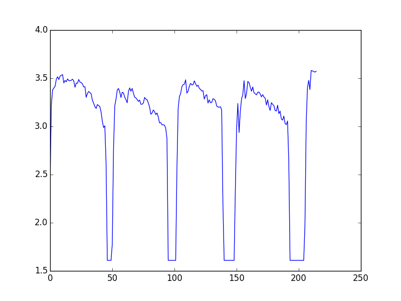
Elle est représentée ici.

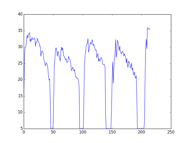
Il semblerait que la différencier une fois suffise à la rendre stationnaire : https://github.com/Vayel/MPF/blob/master/data/views/differenced/8936.pdf

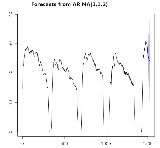
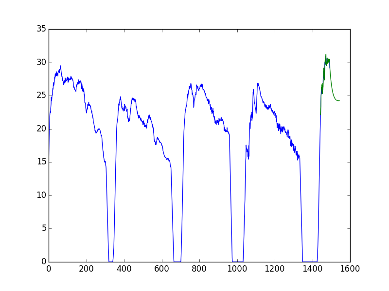
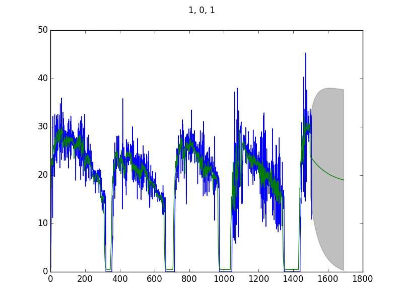
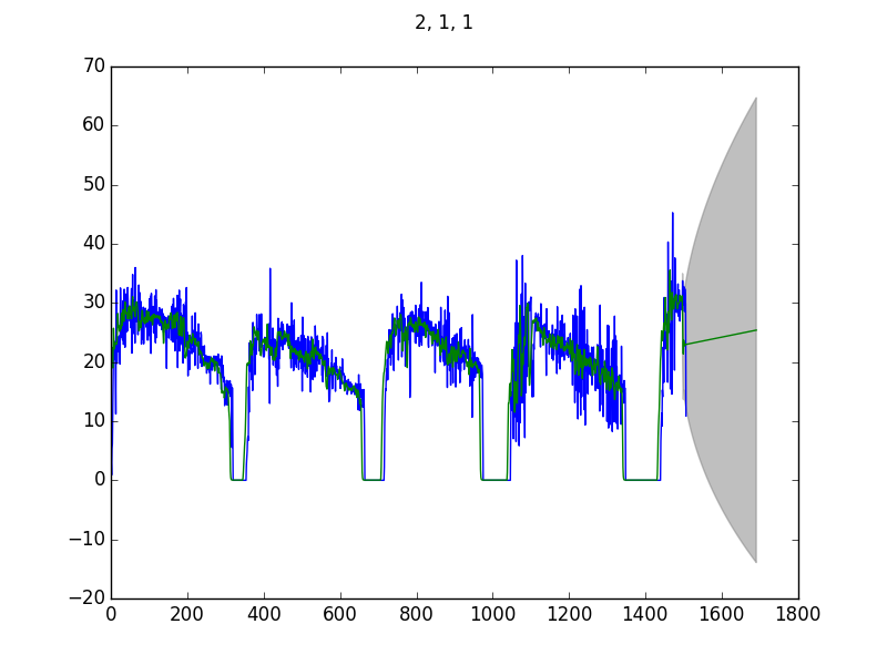
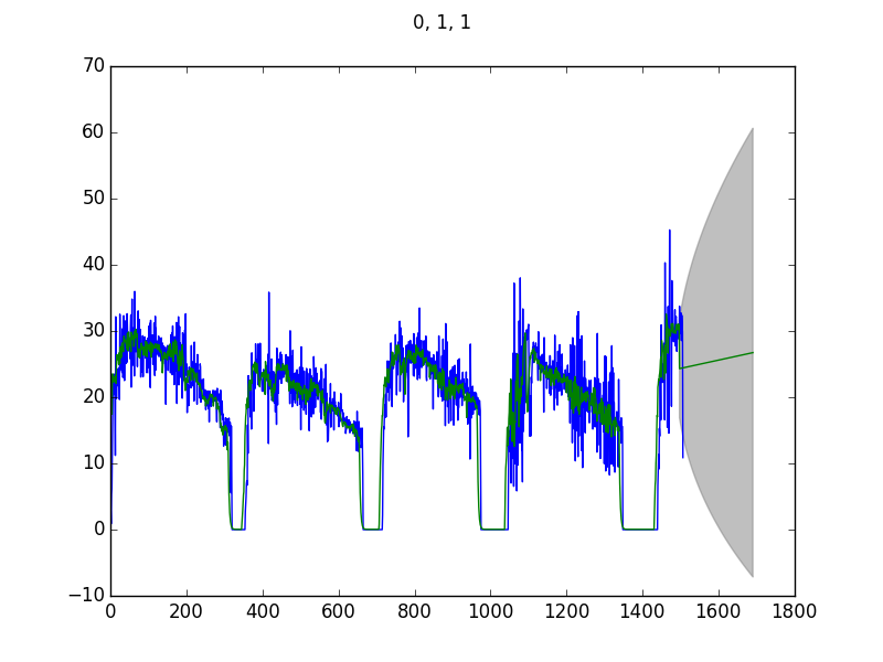
En considérant l'ACF et la PACF, je suis parti sur un modèle ARIMA(1, 1, 1). Dans le doute, j'en ai tracés plusieurs.

101

111

211

011

Le code est le suivant :

 1
 2
 3
 4
 5
 6
 7
 8
 9
10
11
12
13
14
15
16
17
18
19
20
import statsmodels.api as sm

def arma(data, p, d, q, start, end):
    model = sm.tsa.ARIMA(data, (p, d, q)).fit()

    fig, ax = plt.subplots()
    fig.suptitle('{}, {}, {}'.format(p, d, q))
    ax.plot(data)
    ax = model.plot_predict(start, end, ax=ax, plot_insample=False)
    fig.savefig('./arma_({}, {}, {}).png'.format(p, d, q))


start = 10
end = 1700

arma(dta, 1, 0, 1, start, end)
arma(dta, 2, 0, 1, start, end)
arma(dta, 1, 1, 1, start, end)
arma(dta, 0, 1, 1, start, end)
arma(dta, 2, 1, 1, start, end)

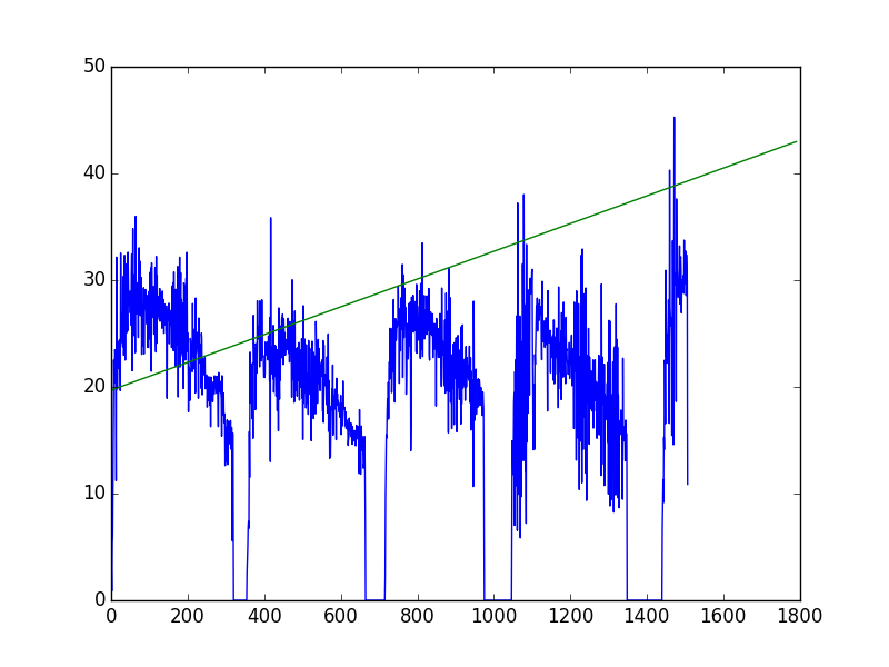
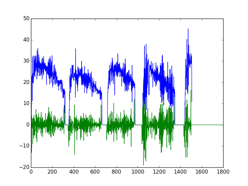
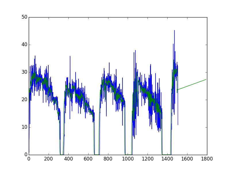
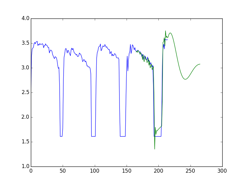
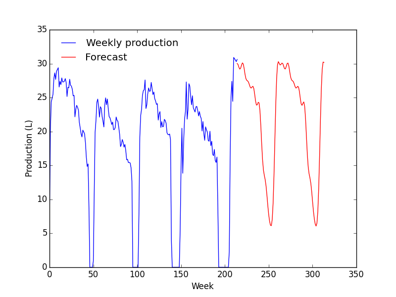
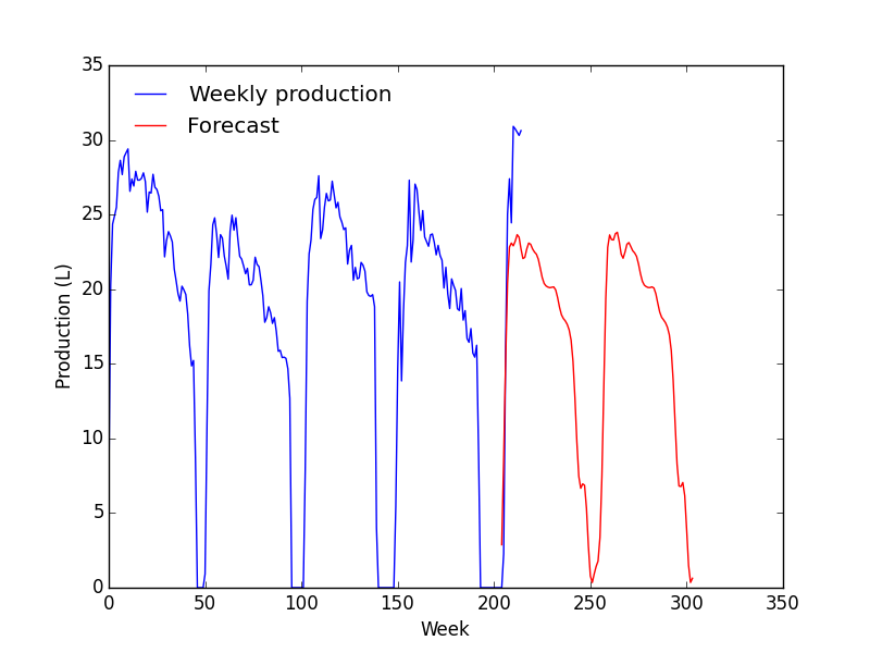
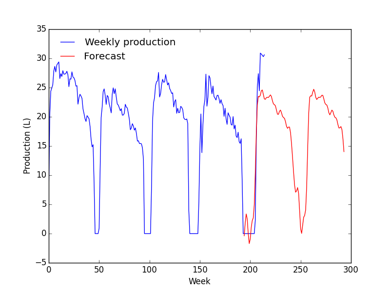
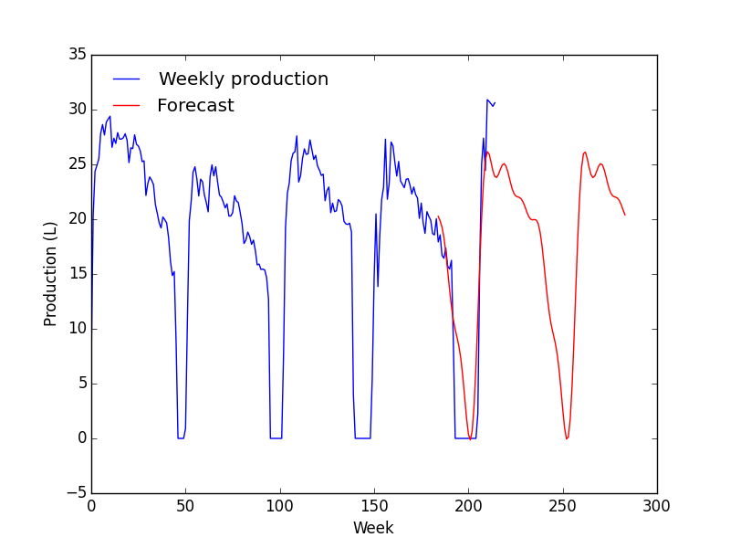
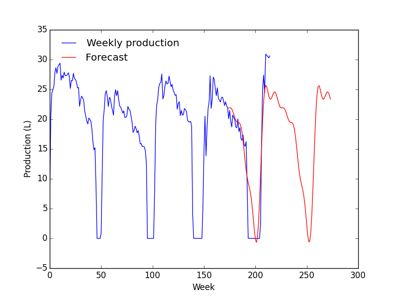
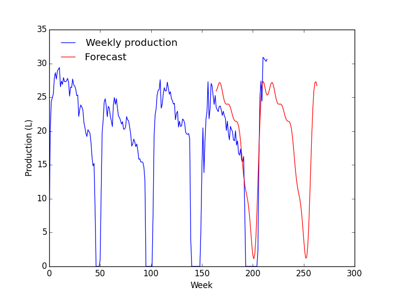
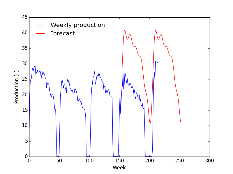
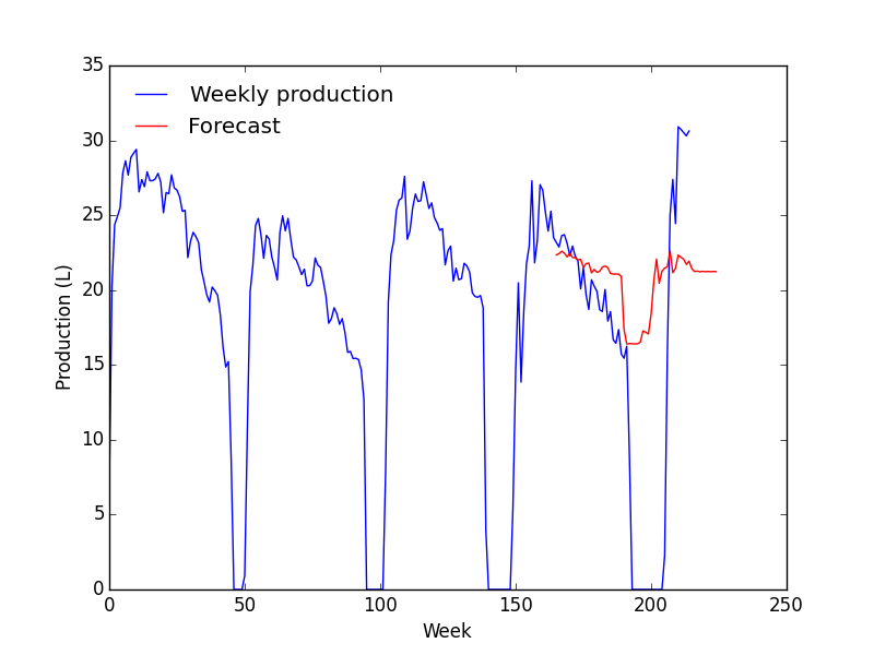
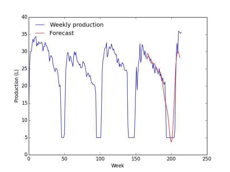
Deux choses me paraissent étranges :

  • Le modèle correspond très bien avec les données mais à partir de la zone de prévision, ça devient n'importe quoi ;
  • La prévision ne change quasiment pas avec les paramètres.

Malheureusement, je ne comprends pas d'où ça peut provenir.

Je me suis inspiré de ça.

Merci !

PS : plot_predict

+1 -0

(Je ne parle pas beaucoup the francais. Je suis un developeur de statsmodels)

Si vous utilize un diff dans le model ARIMA(1, 1, 1), il a besoin de typ=level pour predict http://statsmodels.sourceforge.net/devel/generated/statsmodels.tsa.arima_model.ARIMA.predict.html http://stackoverflow.com/questions/30108091/comparison-of-results-from-statsmodels-arima-with-original-data

Aussi, je crois que vous avez besoin d'une trend pour chaque annee pour la diminuition de la production pendant l'annee. exog en ARIMA.

Josef (J'ai trouve la question par chance avec Google.)

Thanks a lot for this answer! It is incredible that you found this topic.

Unfortunately, the typ parameter appears to be at levels by default. Anyway, the plots coincide on the in-sample values. So I do not understand why the prediction is so approximate.

Concerning the trend, I would be interested in hearing more about it. I suppose that you mean "lactation" (the saisonnality : from calving to drying up) instead of "annee". The problem is that the production first increases then plunges till zero. Then, what is the trend?

Maybe I should remove the saisonnality with a moving average, but differencing the data seems to do the job for having the series stationnary (and being able to use ARIMA). I should use the Dickey-Fuller test to confirm that, but I do not really understand it : https://zestedesavoir.com/forums/sujet/3280/test-de-dickey-fuller-avec-statsmodels/

Thanks again for your support (and sorry for my English).

+0 -0

According to the documentation and the code the default for typ is linear not level.

about the trend:

I think either differencing or explicit modeling of it would work. However, if you difference the series, then there should be a negative intercept, which should result in a downward drift or stochastic trend when you predict in levels.

If you have a relatively regular trend in the seasonal structure (lactation period), then I think modeling it as fixed trend would work better. You could use a low order polynomial or a low order spline (from patsy) to model curvature in the within season trend.

I browsed some of your plots: Are the differences in the seasonal trend between cows inherent to the cows (differences across individuals) or are there some explanatory variables for it.

In general, since you are doing long term forecasting (many periods, days), then it might be useful to think more about trend and deterministic components, than the short term time series behavior with ARIMA with small number of lags. Although, differencing might work quite well for prediction when there is break in the seasonal pattern for a cow, which I guess is caused by some specific events (based on looking at some of your plots).

The problem is there when there are no data to build the prediction. Indeed, with dynamic to True, I have:

Dynamic prediction

Linear prediction:

Linear prediction

Levels prediction (default in plot_predict : https://github.com/statsmodels/statsmodels/blob/master/statsmodels/tsa/arima_model.py#L1834):

Levels prediction

What's strange is that ARIMA works well here. Yet, I followed the same steps.

Concerning the differences, I assume that the seasons depend on the cow. Anyway, I first work on one cow only and lead a univariate analysis (eg: feed influence is not studied). But honestly I do not know how it works. Modelling is one of the targets.

+0 -0

Ok, it wasn't clear to me how you combine different lactation "seasons"

The problem, as briefly discussed in the other thread, is that if you run ARIMA on the entire sample (4 seasons like in the last plot), the drift or intercept in differences is estimated across seasons not within a season. (it's positive in the last plot, I guess)

So, using the current ARIMAX implementation, you cannot estimate a within season intercept directly. There is a seasonal SARIMAX model in statsmodels master, but I think it will be easier to model the seasonal trend directly. Try exog = period_in_season to see if it works better and then you could try a spline with a few knots (degrees of freedom) http://patsy.readthedocs.org/en/latest/spline-regression.html

Oh! You're right! I missed it! In this example, the model is made on one season only.

However, I do not really understand what ARMAX is. exog means that I am trying to explain the production with another variable (eg: feed), doesn't it? But I have no other variable.

Moreover, exog is an array in ARMA.predict. Have I to pass the values of the series during one lactation (I primarily thought that I had to pass the duration of a period)?

+0 -0

exog can be any explanatory variables, the automatically included intercept and trend options are similar to it. exog doesn't have to be a real explanatory variable like feed, but can also just be a dummy variable or trend variable to adjust the mean of the prediction.

You would need to provide the exog for out of sample prediction. exog could just be something like np.arange(day - start_of_season, end_of_season - start_of_season) and you give the corresponding slice for the forecasting period to predict.

In general, the model is that the deviation from the deterministic part is an ARIMA process (y - X * beta) is ARIMA. The exog, X, could be empty, that is have zero intercept, just a constant, or a trend or anything else, like a within season trend.

I am sorry, I did not understand what day is. Does the arange represent the days for the season to predict? Else, whose season are they?

The seasons appear to last the same time:

Lactations

+0 -0

The seasonal trend would be stacking together the numbers from one to about 320, once for each season, exactly the way the x-axis is labeled in the last plot.

The way I thought about this is that day is your concatenated index representing days on record for the cow, say 800 in the previous plot, start of corresponding season is at 700, so the trend period for day 800 would be 100, and would be the same as in your last plot (days since beginning of season).

Adding trend like this would largely correspond to fitting a regression line or curve to your last plot, production as function of day of season pooled over 5 years).

That's strange: passing the exog parameter does not change anything.

 1
 2
 3
 4
 5
 6
 7
 8
 9
10
11
12
13
14
15
16
17
18
19
20
21
22
23
24
import statsmodels.api as sm

def arma(data, p, d, q, start, end, exog):
    model = sm.tsa.ARIMA(data, (p, d, q)).fit()
    predict = model.predict(start=start, end=end, typ='levels', exog=exog, 
        dynamic=True)

    plt.plot(range(len(data)), data)
    plt.plot(range(len(predict)), predict)
    plt.savefig('./arma_({}, {}, {}).png'.format(p, d, q))


dta = mongo.data(_id)
diff_id = diff_ids[LABELS['values']]
diff_dta = mongo.data(diff_id)

durations = [len(mongo.prods(cow, lact)) for lact in mongo.lacts(cow)]
lact_dur = int(sum(durations)/len(durations))
exog = range(lact_dur)

start = 50 
end = 1800

arma(dta, 1, 1, 1, start, end, exog)

The series appears to be stationary:

1
2
3
4
5
>>> sm.tsa.stattools.adfuller(dta)
(-3.8535137605866305, 0.0024048823206302677, 23, 1483, {'5%': -2.8634908922653302, '1%': -3.4347671645756304, '10%': -2.5678086339403325}, 7982.1399270341799)

>>> sm.tsa.stattools.adfuller(diff_dta)
(-7.8470556885881599, 5.7318468331677856e-12, 20, 1485, {'5%': -2.8634882621786728, '1%': -3.4347612052013901, '10%': -2.5678072333888831}, 7985.3887776714364)
+0 -0

It appears to work with R but statsmodels still returns strange forecasts.

 1
 2
 3
 4
 5
 6
 7
 8
 9
10
11
12
13
14
15
16
17
18
19
20
21
import rpy2.robjects as robjects
import rpy2.robjects.packages as rpackages

fcast = rpackages.importr('forecast')
tseries = rpackages.importr('tseries')

plot = robjects.r('plot')
_list = robjects.r('list')
c = robjects.r('c')
diff = robjects.r('diff')
ts = robjects.r('ts')

# dta is a list containing the productions of one cow
dta = robjects.r('as.numeric')(dta)
model = fcast.auto_arima(ts(dta), stepwise=False, 
                         approximation=False)
# The previous line gives an ARIMA(3, 1, 2)
# The seasonnality seems not to be taken into account
fit = fcast.Arima(dta, order=c(3, 1, 2))
forecast = fcast.forecast_Arima(fit, 30)
plot(forecast) 

ARIMA(3, 1, 2) with R

Will work on a seasonal model these days.

+0 -0

statsmodels gives the same forecasts as R with an ARIMA(3, 1, 2) model.

ARIMA(3, 1, 2)

But I cannot figure out why the seasonality does not appear in the automatic model. I even tried an STL decomposition with R but it gave me an error: la série n'est pas périodique ou elle a moins de deux périodes. In English: the series is not seasonal or has fewer than two seasons. Yet, it appears to have four.

Thanks.

+0 -0

The seasonality is not taken into account but I managed to improve the model.

  • Dwindle the number of points and shift the data to apply log

Weekly data

 1
 2
 3
 4
 5
 6
 7
 8
 9
10
11
12
13
14
15
16
17
18
19
20
def change_period(data, period):
    """Change the period of the series. The series is not altered.

    :param data: The values of the series.
    :param period: The new period.

    :type data: list
    :type period: int

    :return: The number of periods and the new series.
    :rtype: tuple
    """

    n = int(len(data)/period)
    series = [sum(data[i*period:(i+1)*period])/period for i in range(n)]

    return n, series


n, data = change_period(data, 7)
  • Take the log to stabilize the variance

Log

  • Look for a model forecast.auto.arima (R function)
 1
 2
 3
 4
 5
 6
 7
 8
 9
10
import rpy2.robjects as robjects
import rpy2.robjects.packages as rpackages

fcast = rpackages.importr('forecast')
ts = robjects.r('ts')

rdata = robjects.r('as.numeric')(log_data)
rdata = ts(rdata)
model = fcast.auto_arima(rdata, stepwise=False, approximation=False, seasonal=True)
# Returns: ARIMA(2, 0, 2)
  • Fit the model to the log data

Forecasts - ARIMA(2, 0, 2)

 1
 2
 3
 4
 5
 6
 7
 8
 9
10
11
12
13
14
15
16
def arma(data, p, d, q, start, end):
    model = sm.tsa.ARIMA(data, (p, d, q)).fit()

    if d: # ARIMA model
        predict = model.predict(start, end, typ='levels')
    else: # ARMA model
        predict = model.predict(start, end)

    plt.plot(range(len(data)), data)
    plt.plot(range(start, end+1), predict)
    plt.savefig('experiments/arima({}, {}, {}).png'.format(p, d, q))
    plt.clf()


fcast_dur = 50
arma(log_data, 2, 0, 2, len(log_data) - fcast_dur, len(log_data) + fcast_dur)

About the seasonality, I found that.

+0 -0

As explained there, the problem with R is due to the size of the seasonal period (about 300 days here).

So I proceeded like that.

 1
 2
 3
 4
 5
 6
 7
 8
 9
10
11
12
13
14
15
16
17
18
19
20
21
22
23
24
25
26
27
28
29
30
31
32
33
34
35
36
37
38
39
40
41
42
43
44
45
46
47
48
49
50
51
52
53
54
55
56
57
58
59
60
61
import rpy2.robjects as robjects
import rpy2.robjects.packages as rpackages
import matplotlib.pyplot as plt
import numpy as np

fcast = rpackages.importr('forecast')


def get_aicc(fit):
    for item in fit.items():
        if 'aicc' in item:
            return item[-1][0]

    return None

def get_best_fit(dta):
    best_K = 1
    best_fit = fcast.auto_arima(dta, xreg=fcast.fourier(dta, K=best_K), seasonal=False)
    best_aicc = get_aicc(best_fit)

    for K in range(2, 15):
        fit = fcast.auto_arima(dta, xreg=fcast.fourier(dta, K=K), seasonal=False)
        aicc = get_aicc(fit)

        if aicc < best_aicc:
            best_fit = fit
            best_aicc = aicc
            best_K = K

    return best_fit, best_K

def get_fcast_vals(fc):
    """Only because I don't know how to get 
    them from the R list vector directly.
    """

    fc = str(fc).split('\n')
    fc = fc[1:-1] # Remove labels and empty string

    return [float(line.split()[1]) for line in fc]

def main(): 
    period = 7
    n, data = tools.change_period(data, period)

    freq = lact_dur/period
    h = 100 # Number of forecasts

    rdata = data.tolist()
    rdata = robjects.r('as.numeric')(rdata)
    rdata = ts(rdata, freq=freq)

    fit, K = get_best_fit(rdata)

    fc = fcast.forecast(fit, xreg=fcast.fourierf(rdata, K=K, h=h))
    fc = get_fcast_vals(fc)

    # Plot
    plt.plot(range(len(data)), data, label='Weekly production')
    plt.plot(range(len(data), len(data) + h), fc, 'r', label='Forecast')
    plt.show()

Not perfect but far better than before.


J'expliquerai tout ça en français ultérieurement. N'hésitez pas à me rappeler à l'ordre si nécessaire.

+0 -0

Je prends enfin le temps de détailler.


On part de la production quotidienne d'une vache :

Production quotidienne

Mais :

On va donc travailler sur des données hebdomadaires :

Production hebdomadaire

Puis on utilise R pour calculer notre modèle SARIMA et prévoir :

SARIMA

 1
 2
 3
 4
 5
 6
 7
 8
 9
10
11
12
13
import rpy2.robjects as robjects


fcast = rpackages.importr('forecast')
ts = robjects.r('ts')


freq = get_season_len(weekly_data)
rdata = robjects.r('as.numeric')(weekly_data)
rdata = ts(rdata, freq=freq)

fit = fcast.auto_arima(rdata)
fc = fcast.forecast(fit, h=fcast_dur)

C'est mauvais. La saisonnalité semble peu prise en compte. Cela est probablement dû à la période de tarissement, où la production forme un pallier à 0. Je ne l'ai pas fait, mais on pourrait enlever ces palliers et les gérer à part. Là, on utilise la transformée de Fourier, comme indiqué dans le lien précédent :

Fourier + ARIMA

 1
 2
 3
 4
 5
 6
 7
 8
 9
10
11
12
13
14
15
16
17
18
19
def get_best_fit(dta):
    best_K = 1
    best_fit = fcast.auto_arima(dta, xreg=fcast.fourier(dta, K=best_K), seasonal=False)
    best_aicc = get_aicc(best_fit)

    for K in range(2, 15):
        fit = fcast.auto_arima(dta, xreg=fcast.fourier(dta, K=K), seasonal=False)
        aicc = get_aicc(fit)

        if aicc < best_aicc:
            best_fit = fit
            best_aicc = aicc
            best_K = K

    return best_fit, best_K


fit, K = get_best_fit(rdata)
fc = fcast.forecast(fit, xreg=fcast.fourierf(rdata, K=K, h=fcast_dur))

C'est bien mieux, même si ce n'est pas l'idéal au niveau de la période de tarissement.

+0 -0
Connectez-vous pour pouvoir poster un message.
Connexion

Pas encore membre ?

Créez un compte en une minute pour profiter pleinement de toutes les fonctionnalités de Zeste de Savoir. Ici, tout est gratuit et sans publicité.
Créer un compte